Across-Trials Within Session Testing with glhmm toolbox#
In this tutorial, we are going to look at how to implement the across trials within sessions testing using the glhmm toolbox. This test is used to assess effect differences between trials in one or more experimental sessions and is therefore ideal to see trial by trial variability within a session.
In the real world scenarios, one would typically fit a Hidden Markov Model (HMM) to an actual dataset. However, for the sake of showing the concept of statistical testing, we just use synthetic data for both the independent variable and the dependent variable for the across_trials_within_session test.
We create synthetic data using the toolbox Genephys, developed by Vidaurre in 2023 (accessible at https://doi.org/10.7554/eLife.87729.2). Genephys makes it possible to simulate electrophysiological data in the context of a psychometric experiment. Hence, it can create scenarios where, for example, a subject is exposed to one or multiple stimuli while simultaneously recording EEG or MEG data.
While the process of preparing the data requires some explanation, executing the test (across_trials_within_session) itself is straightforward —simply input the variables D and R, and define the specific method you wish to apply. The methods include permutation using regression or permutation using correlation and is described in the paper Vidaurre et al.
2023.
Table of Contents#
Load and prepare data
Look at data
Prepare data for HMM
Load or initialise and train HMM
Data restructuring
Across-trials within session testing
Across-trials within sessions testing - Regression
Across-trials within sessions testing - Correlation
Install necessary packages#
Let’s start by importing the required libraries and modules.
First, we will need to import the GLHMM-package as glhmm:
If you dont have the GLHMM-package installed, then run the following command in your terminal:
pip install --user git+https://github.com/vidaurre/glhmm
To use the function glhmm.statistics.py you also need to install the library’s:
pip install statsmodels
pip install tqdm
python -m pip install -U scikit-image
```
Import libraries#
Let’s start by importing the required libraries and modules.
[85]:
import os
import numpy as np
import glhmm.glhmm as glhmm
import glhmm.graphics as graphics
import glhmm.preproc as preproc
import glhmm.statistics as statistics
import glhmm.auxiliary as auxiliary
import glhmm.io as io
1. Load and prepare data#
[86]:
# Get the current directory
current_directory = os.getcwd()
folder_name = "\\data_statistical_testing"

# Load D data
file_name = '\\D_trials.npy'
file_path = os.path.join(current_directory+folder_name+file_name)
D_trials = np.load(file_path)

# Load R data
file_name = '\\R_trials.npy'
file_path = os.path.join(current_directory+folder_name+file_name)
R_trials = np.load(file_path).astype(int)


# Load indices
file_name = '\\idx_trials_session.npy'
file_path = os.path.join(current_directory+folder_name+file_name)
idx_trials_session = np.load(file_path)


# Load time indices for every trial
file_name = '\\idx_trials.npy'
file_path = os.path.join(current_directory+folder_name+file_name)
idx_trials = np.load(file_path)


print(f"Data dimension of D-session data: {D_trials.shape}")
print(f"Data dimension of R-session data: {R_trials.shape}")
print(f"Data dimension of indices for each trial: {idx_trials_session.shape}")
print(f"Data dimension of indices: {idx_trials.shape}")
Data dimension of D-session data: (250, 1421, 16)
Data dimension of R-session data: (1421,)
Data dimension of indices for each trial: (10, 2)
Data dimension of indices: (1421, 2)
Look at data#
Now we can look at the data structure. - D_sessions: 3D array of shape (n_timepoints, n_trials, n_features) - R_sessions: 3D array of shape (n_trials,) - idx_data: 2D array of shape (n_sessions, 2)
D_sessions represents the data collected from the subject, structured as a list with three elements: [250, 1421, 16]. The first element indicates that the subject underwent measurement across 250 timepoints. The second element, 1421 corresponds to the total number of trials conducted. In this context, 10 distinct sessions were executed, each comprising 150 trials, lead up to a total of 1421 trials (150*10). Each individual trial involved the measurement of 16 channels within the EEG or
MEG scanner.
R_sessions categorial values of when a stimulus is prestented. It contain values of 1 and 2.
idx_trials_session.shape = [10, 2] shows the indices for the number of sessions conducted, which in this case is 10 The values in each row represent the indices for the first and last trial for a given session. As you can see the number of trials are different from each session.
np.diff(idx_trials_session)
array([[129],
       [132],
       [150],
       [150],
       [150],
       [150],
       [150],
       [150],
       [111],
       [149]])
Lastly, we have idx_trials.shape = [1421, 2], which marks the number of trials conducted, which in this case is 1421 The values in each row represent the start and end indices for every trial. Having this index to seperate the time period for each trial is required when training a time-delay embedded HMM (TDE-HMM).
Prepare data for HMM#
When you’re getting into training a Hidden Markov Model (HMM), the input data needs to follow a certain setup. The data shape should look like ((number of timepoints * number of trials), number of features). This means you’ve lined up all the trials from different sessions side by side in one long row. The second dimension is the number of features, which could be the number of parcels or channels.
So, in our scenario, we’ve got this data matrix, D_session, shaped like [250, 1421, 16] (timepoints, trials, channels). Now, when we bring all those trials together, it’s like stacking them up to create a new design matrix, and it ends up with a shape of [355250, 16] (timepoints * trials, channels). Beside that we also need to update R_session and idx_trials_session to sync up with the newly concatenated data. To make life easier, we’ve got the function
get_concatenate_sessions. It does the heavy lifting for us.
Note: it is important to use ``idx_trials_session`` for this function as the concatenation is done trial-by-trial basis for every defined session.
[87]:
D_con,R_con,idx_con=statistics.get_concatenate_sessions(D_trials, R_trials, idx_trials_session)
print(f"Data dimension of the concatenated D-data: {D_con.shape}")
print(f"Data dimension of the concatenated R-data: {R_con.shape}")
print(f"Data dimension of the updated time stamp indices: {idx_con.shape}")
Data dimension of the concatenated D-data: (355250, 16)
Data dimension of the concatenated R-data: (355250,)
Data dimension of the updated time stamp indices: (10, 2)
For a quick sanity check, let’s verify whether the concatenation was performed correctly on D_trials. We’ve essentially stacked up every timepoint from each trial sequentially.
D_trials[:, 0, :], with the corresponding slice in the concatenated data, D_con[0:250, :].D_trials[:, 0, :] == D_con[0:250, :] holds true, we’re essentially confirming that all timepoints in the first trial align perfectly with the first 250 values in our concatenated data. It’s like double-checking to make sure everything lined up as expected.[88]:
D_trials[:,0,:]==D_con[0:250,:]
[88]:
array([[ True,  True,  True, ...,  True,  True,  True],
       [ True,  True,  True, ...,  True,  True,  True],
       [ True,  True,  True, ...,  True,  True,  True],
       ...,
       [ True,  True,  True, ...,  True,  True,  True],
       [ True,  True,  True, ...,  True,  True,  True],
       [ True,  True,  True, ...,  True,  True,  True]])
Here, it’s evident that the concatenation process has been executed accurately.
Next up, let’s confirm if the values in idx_con have been appropriately updated. Each row in this matrix should represent the total count of timepoints and trials for each of the 10 sessions.
[89]:
idx_con
[89]:
array([[     0,  32250],
       [ 32250,  65250],
       [ 65250, 102750],
       [102750, 140250],
       [140250, 177750],
       [177750, 215250],
       [215250, 252750],
       [252750, 290250],
       [290250, 318000],
       [318000, 355250]])
Indeed, each session now aligns with the number of datapoints. This means that when we pooled together the timepoints and trials, the count for each session ended up exactly as expected. It’s a reassuring confirmation that our concatenation didn’t miss a beat.
2. Load data or initialise and train HMM#
You can either load the Gamma values from a pretrained model or train your own model. If you prefer the former option, load the data (Gamma_trials) from the data_statistical_testing folder. In this example we have trained a TDE-HMM, incorporating mean and covariance parameters for 6 distinct states. TDE-HMM calculates the covariance and then compares the covariance at different time points. If the
covariances are similar, the time points are assigned to the same state; otherwise, they are assigned to different states.
current_directory = os.getcwd()
folder_name = "\\data_statistical_testing"

# Load Gamma data
file_name = '\\Gamma_trials.npy'
file_path = os.path.join(current_directory+folder_name+file_name)
Gamma_tde = np.load(file_path)
print(f"Data dimension of Gamma: {Gamma_tde.shape}")
If you decide to train your own TDE-HMM model, you need to prepare the dataset by adding lags that act like a sliding window. These lags capture temporal dependencies in the data and span from -n to n, passing through zero. The code below shows how to define such lags:
# Create lag array
lag_val =list(range(-7, 8, 1))
print(lag_val)
[-7, -6, -5, -4, -3, -2, -1, 0, 1, 2, 3, 4, 5, 6, 7]
Once the dataset is appropriately prepared, you can proceed with training the TDE-HMM.
[91]:
# Define the number of lags (Window size)
lag_val =list(range(-7, 8, 1))
preproc.build_data_tde, so it is ready for the TDE-HMM.D_con), the indices that defines the running period for each trial (idx_trials) of the concatenated data, and the lag kernel (lag_val) that will run over each trial.[92]:
idx_trials
[92]:
array([[     0,    250],
       [   250,    500],
       [   500,    750],
       ...,
       [354500, 354750],
       [354750, 355000],
       [355000, 355250]])
[93]:
# Prepare the dataset for TDE-HMM
D_con_tde,idx_tde = preproc.build_data_tde(D_con, idx_trials,lag_val)
[94]:
print(f"Data dimension of the concatenated TDE D-data: {D_con_tde.shape}")
print(f"Data dimension of the updated TDE time stamp indices: {idx_tde.shape}")
Data dimension of the concatenated TDE D-data: (335356, 240)
Data dimension of the updated TDE time stamp indices: (1421, 2)
Upon examination, you’ll notice that the dimension of the concatenated TDE D-data has undergone a transformation from (355250, 16) to (335356, 240).
This transformation is a result of the specified kernel size for the lag, applied individually to each trial. The defined lag kernel ranges from -7 to 7, indicating that we have pooled/excluded 7 data points from both the beginning and end of each trial. In essence, the original trial length of 250 time points has been reduced to 236 (250 - 14).
This adjustment applies for all 1421 trials in our dataset. Initially, the total number of data points in the concatenated data was 355250 (1421 * 250), as indicated at the beginning of this notebook when we loaded the data. However, after processing, D_con_tde now contains 335356 data points, equivalent to 1421 * 236.
If look into idx_tde, we can see that the number period for each trial are 236 points, which match with the pooled 7 data points from both the beginning and end of each trial based on the defined lag_val
Checking out idx_tde, you’ll notice that each trial now spans 236 points, matching the 7 pooled data points from both ends based on the specified kernel size of lag_val.
[95]:
idx_tde
[95]:
array([[     0,    236],
       [   236,    472],
       [   472,    708],
       ...,
       [334648, 334884],
       [334884, 335120],
       [335120, 335356]])
Initialize-HMM#
If you want to train your own HMM you need to do the following steps. First, we need to initialize the hmm object and set the hyperparameters according to our modeling preferences.
In this case, we choose not to model an interaction between two sets of variables in the HMM states, so we set model_beta='no'. For our estimation, we choose K=6 states. If you wish to model a different number of states, simply adjust the value of K.
Our modeling approach involves representing states as Gaussian distributions with mean and a full covariance matrix. This means that each state is characterized by a mean amplitude and a functional connectivity pattern. To specify this configuration, set covtype='full'. If you prefer not to model the mean, you can include model_mean='no'. Optionally, you can check the hyperparameters to make sure that they correspond to how you want the model to be set up.
[96]:
# Create an instance of the glhmm class
K = 6 # number of states
hmm = glhmm.glhmm(model_beta='no', K=K, covtype='full')
print(hmm.hyperparameters)
{'K': 6, 'covtype': 'full', 'model_mean': 'state', 'model_beta': 'no', 'dirichlet_diag': 10, 'connectivity': None, 'Pstructure': array([[ True,  True,  True,  True,  True,  True],
       [ True,  True,  True,  True,  True,  True],
       [ True,  True,  True,  True,  True,  True],
       [ True,  True,  True,  True,  True,  True],
       [ True,  True,  True,  True,  True,  True],
       [ True,  True,  True,  True,  True,  True]]), 'Pistructure': array([ True,  True,  True,  True,  True,  True])}
Train an HMM#
Now, let’s proceed to train the TDE-HMM using the data (D_con_tde) and time indices (idx_tde).
Since in this case, we are not modeling an interaction between two sets of timeseries but opting for a “classic” HMM, we set X=None. For training, Y should represent the timeseries from which we aim to estimate states (D_con_tde), and indices should encompass the beginning and end indices of each subject (idx_tde).
[97]:
Gamma_tde,Xi,FE = hmm.train(X=None, Y=D_con_tde, indices=idx_tde)
Init repetition 1 free energy = 116160832.74711715
Init repetition 2 free energy = 116184285.88186334
Init repetition 3 free energy = 116178456.68257196
Init repetition 4 free energy = 116166816.5333639
Init repetition 5 free energy = 116175886.17767626
Best repetition: 1
Cycle 1 free energy = 116160746.57477993
Cycle 2 free energy = 116156394.67067881
Cycle 3, free energy = 116154895.40152383, relative change = 0.2562339362311568
Cycle 4, free energy = 116153783.89172213, relative change = 0.15963814415702063
Cycle 5, free energy = 116152863.28739019, relative change = 0.11677924277358287
Cycle 6, free energy = 116152084.07307974, relative change = 0.08995257229617734
Cycle 7, free energy = 116151384.80602844, relative change = 0.07469390345530229
Cycle 8, free energy = 116150759.78463948, relative change = 0.06258481255466751
Cycle 9, free energy = 116150237.40955001, relative change = 0.049706620653324596
Cycle 10, free energy = 116149776.78566559, relative change = 0.041990222384711076
Cycle 11, free energy = 116149364.76900281, relative change = 0.03619958650188911
Cycle 12, free energy = 116148972.92359719, relative change = 0.033281553830788325
Cycle 13, free energy = 116148611.40985, relative change = 0.029790591992198114
Cycle 14, free energy = 116148270.01262315, relative change = 0.027363084683515528
Cycle 15, free energy = 116147936.3199885, relative change = 0.02604886788555741
Cycle 16, free energy = 116147622.7208431, relative change = 0.02389535474161959
Cycle 17, free energy = 116147303.75488736, relative change = 0.02372760762237403
Cycle 18, free energy = 116146981.17573616, relative change = 0.023434057390751332
Cycle 19, free energy = 116146674.47741492, relative change = 0.021794783910522766
Cycle 20, free energy = 116146371.71899211, relative change = 0.021061666793452186
Cycle 21, free energy = 116146109.25348896, relative change = 0.017931252442897942
Cycle 22, free energy = 116145860.88547014, relative change = 0.016685019662309043
Cycle 23, free energy = 116145609.47066496, relative change = 0.016609174599342563
Cycle 24, free energy = 116145380.68378504, relative change = 0.014889268705796585
Cycle 25, free energy = 116145149.78708827, relative change = 0.01480411872791112
Cycle 26, free energy = 116144920.28213765, relative change = 0.014501497970191363
Cycle 27, free energy = 116144713.60652064, relative change = 0.012890664639696323
Cycle 28, free energy = 116144502.05839881, relative change = 0.013022740527431069
Cycle 29, free energy = 116144301.45314702, relative change = 0.012198465676758327
Cycle 30, free energy = 116144116.46908307, relative change = 0.01112344487312083
Cycle 31, free energy = 116143958.37975559, relative change = 0.009416695913715217
Cycle 32, free energy = 116143801.04031198, relative change = 0.009285009210343805
Cycle 33, free energy = 116143662.98354504, relative change = 0.008081249723428618
Cycle 34, free energy = 116143539.59148137, relative change = 0.007171045704029469
Cycle 35, free energy = 116143421.58868587, relative change = 0.006811133634503649
Cycle 36, free energy = 116143316.40447883, relative change = 0.006034605813948098
Cycle 37, free energy = 116143209.34806436, relative change = 0.006104523606064881
Cycle 38, free energy = 116143101.62979405, relative change = 0.006104766572120824
Cycle 39, free energy = 116142995.5464166, relative change = 0.005976182071222325
Cycle 40, free energy = 116142883.74259001, relative change = 0.006259020148468852
Cycle 41, free energy = 116142771.13466519, relative change = 0.00626454340479123
Cycle 42, free energy = 116142669.30051611, relative change = 0.005633269020063474
Cycle 43, free energy = 116142570.7915425, relative change = 0.0054197924967839765
Cycle 44, free energy = 116142486.87957822, relative change = 0.004595474533142033
Cycle 45, free energy = 116142410.70759594, relative change = 0.004154261236141418
Cycle 46, free energy = 116142328.08621898, relative change = 0.004485784850808166
Cycle 47, free energy = 116142240.77240023, relative change = 0.004718186056528753
Cycle 48, free energy = 116142160.27877961, relative change = 0.004330804836951164
Cycle 49, free energy = 116142074.45831496, relative change = 0.004596183020642024
Cycle 50, free energy = 116141986.67349267, relative change = 0.0046793861513973745
Cycle 51, free energy = 116141900.44536145, relative change = 0.0045753761584171
Cycle 52, free energy = 116141812.76842976, relative change = 0.004630708166789479
Cycle 53, free energy = 116141726.5323046, relative change = 0.0045339607031974795
Cycle 54, free energy = 116141641.80092287, relative change = 0.004435089489318731
Cycle 55, free energy = 116141565.53385688, relative change = 0.003976169296180571
Cycle 56, free energy = 116141499.5687752, relative change = 0.003427290543820727
Cycle 57, free energy = 116141439.23050363, relative change = 0.0031251460951711666
Cycle 58, free energy = 116141377.7343941, relative change = 0.0031750021325663426
Cycle 59, free energy = 116141320.46528657, relative change = 0.0029480482211354116
Cycle 60, free energy = 116141264.21385422, relative change = 0.002887300597644794
Cycle 61, free energy = 116141205.6943079, relative change = 0.002994724133015651
Cycle 62, free energy = 116141143.42748977, relative change = 0.003176368426938569
Cycle 63, free energy = 116141080.49509944, relative change = 0.0032000475618261057
Cycle 64, free energy = 116141016.45087858, relative change = 0.003246012097287603
Cycle 65, free energy = 116140934.30808872, relative change = 0.004146057144084983
Cycle 66, free energy = 116140858.55458456, relative change = 0.0038090017715650373
Cycle 67, free energy = 116140796.46810387, relative change = 0.003112087654475641
Cycle 68, free energy = 116140743.35277481, relative change = 0.0026553386771090643
Cycle 69, free energy = 116140697.4604658, relative change = 0.002288994331170984
Cycle 70, free energy = 116140656.09010112, relative change = 0.0020592019228152974
Cycle 71, free energy = 116140609.21567175, relative change = 0.0023277346906870632
Cycle 72, free energy = 116140548.46245335, relative change = 0.0030078661518065306
Cycle 73, free energy = 116140496.47233486, relative change = 0.0025674002701816952
Cycle 74, free energy = 116140450.7249924, relative change = 0.0022540244900417193
Cycle 75, free energy = 116140407.35619111, relative change = 0.0021322747032527325
Cycle 76, free energy = 116140366.4018087, relative change = 0.002009520845450753
Cycle 77, free energy = 116140324.888154, relative change = 0.0020328220413124336
Cycle 78, free energy = 116140288.33593163, relative change = 0.0017866749255467263
Cycle 79, free energy = 116140255.57571703, relative change = 0.0015987612168851038
Cycle 80, free energy = 116140220.10792896, relative change = 0.001727905163999072
Cycle 81, free energy = 116140178.85139069, relative change = 0.002005887452448486
Cycle 82, free energy = 116140135.28048724, relative change = 0.002113933401344278
Cycle 83, free energy = 116140095.2162508, relative change = 0.0019400290966726933
Cycle 84, free energy = 116140059.20730874, relative change = 0.0017406246646787457
Cycle 85, free energy = 116140020.39582665, relative change = 0.0018725826006942212
Cycle 86, free energy = 116139982.82920367, relative change = 0.0018092411530189656
Cycle 87, free energy = 116139949.08947429, relative change = 0.0016222985076711197
Cycle 88, free energy = 116139909.11382177, relative change = 0.0019184512257116942
Cycle 89, free energy = 116139868.38153568, relative change = 0.0019509488018959607
Cycle 90, free energy = 116139828.86736621, relative change = 0.0018890296478457215
Cycle 91, free energy = 116139791.31623438, relative change = 0.0017919670018863947
Cycle 92, free energy = 116139749.15294811, relative change = 0.0020080220613000683
Cycle 93, free energy = 116139704.05432737, relative change = 0.0021432138247999164
Cycle 94, free energy = 116139660.38922814, relative change = 0.0020707917572923592
Cycle 95, free energy = 116139613.9653456, relative change = 0.0021967889329247894
Cycle 96, free energy = 116139566.15619923, relative change = 0.00225723331162292
Cycle 97, free energy = 116139521.28880166, relative change = 0.002113865397267175
Cycle 98, free energy = 116139475.71970008, relative change = 0.0021423257974812772
Cycle 99, free energy = 116139430.86500917, relative change = 0.002104302009728437
Cycle 100, free energy = 116139387.98224562, relative change = 0.0020077523123685336
Finished training in 18460.39s : active states = 6
Now, checking out Gamma, you’ll see it’s got the same number of points as the concatenated dataset (335356 ). Each column in Gamma stands for one of the six different states.
[64]:
Gamma_tde.shape
[64]:
(335356, 6)
auxiliary.padGamma function, which takes Gamma, T, and option as inputs. * Gamma: This is the Gamma we obtained from the TDE-HMM. * T: Represents the desired number of data points for each trial, which needs to go back from 236 to 250. We can obtain T using the auxiliary.get_T function, which requires the original indices idx_trials as input. * option: A
dictionary where the key can be either “embeddedlags” or “order”. Since we’re using lags in this case, we set the key to “embeddedlags,” and the value is the variable lag_val.[65]:
# Get T
T = auxiliary.get_T(idx_trials)
# Define options
options ={'embeddedlags':lag_val}
Gamma =auxiliary.padGamma(Gamma_tde,T,options=options)
Look at Gamma
[66]:
#Look at shape for Gamma and D_con
Gamma.shape, D_con.shape
[66]:
((355250, 6), (355250, 16))
Now, you’ll notice that the number of data points in both Gamma and D_con are back in sync.
Taking a closer look at the padding for the initial trial in state 1, you can observe that padding has been applied to the first 7 data points and the last 7 data points.
[67]:
# As we can see the padding works, since the first and last 7 numbers
# has been added to the timepoints for every trial
Gamma[:10,0].round(3),Gamma[240:250,0].round(3)
[67]:
(array([0.358, 0.358, 0.358, 0.358, 0.358, 0.358, 0.358, 0.   , 0.   ,
        0.   ]),
 array([0.968, 0.998, 0.999, 0.358, 0.358, 0.358, 0.358, 0.358, 0.358,
        0.358]))
Data restructuring#
Now we have trained our HMM and got our Gamma values we need to restructure the data back to the original data structure. In this case we are not doing HMM-aggregated statistics, but we will instead perform the statistical testing per time point. We will acheive this by applying the function reconstruct_concatenated_design. It takes a concatenated 2D matrix and converts it into a 3D matrix. So, it will convert Gamma, shaped like [355250, 6] back to the original format for number
of time points and trials shaped like [250, 1421, 6] (timepoints, trials, states).
[68]:
# Reconstruct the Gamma matrix
n_timepoints, n_trials, n_channels = D_trials.shape[0],D_trials.shape[1],Gamma.shape[1]
Gamma_reconstruct =statistics.reconstruct_concatenated_design(Gamma,n_timepoints=n_timepoints, n_trials=n_trials, n_channels=n_channels)
Gamma_reconstruct.shape
[68]:
(250, 1421, 6)
As a sanity check we will see if Gamma_reconstruct is actually structured correctly by comparing it with Gamma.
Gamma_reconstruct[:, 0, :], with the corresponding slice in the concatenated 2D-data, Gamma[0:250, :].Gamma_reconstruct[:, 0, :] == Gamma[0:250, :] holds true, we’re essentially confirming that all timepoints in the first trial align perfectly with the first 250 values in our concatenated data.[69]:
Gamma_reconstruct[:, 0, :] == Gamma[0:250, :]
[69]:
array([[ True,  True,  True,  True,  True,  True],
       [ True,  True,  True,  True,  True,  True],
       [ True,  True,  True,  True,  True,  True],
       ...,
       [ True,  True,  True,  True,  True,  True],
       [ True,  True,  True,  True,  True,  True],
       [ True,  True,  True,  True,  True,  True]])
What we can see here is that all the values are True and we therefore know that the restructuring is performed correctly.
3. Across-trials within session testing#
As we move on to the next part of this tutorial, let’s dive into how we can use the across_trials_within_subject function. This function helps us to find connections between HMM state occurrences (D) and behavioral variables or individual traits (R) using permutation testing.

Figure 5C in Vidaurre et al. 2023: A 9 x 4 matrix representing permutation testing across trials. Each number corresponds to a trial within a session, and permutations are performed within sessions.
Hypothesis * Null Hypothesis (H0): No significant relationship exists between the independent variables and the dependent variable. * Alternative Hypothesis (H1): There is a significant relationship between the independent variables and the dependent variable.
Across-trials within sessions testing - Regression#
In regression analysis, we are trying to explain the relationships between predictor variables (D) the response variable (R). Our goal is to identify the factors that contribute to changes in our signal over time. The permutation test for explained variance assess the statistical significance of relationships between state time courses (D) and behavioral measurements (R). A significant result indicates that certain patterns within the state time courses (Gamma_reconstruct) significantly
contribute in explaining why the behavioral measurements varies across trials. A non-significant result suggests that he state time courses may not play a role in accounting for the variability of the behavioral measurements.
across_trials_within_session function, input the variables Gamma_reconstruct (D) and R_trials (R). Additionally, you can account for potential confounding variables by regressing them out through permutation testing. Initiating regression-based permutation testing involves setting method="regression". For an in-depth comprehension of the function look at the documentation.[71]:
import statistics_new as statistics
# Set the parameters for across sessions within subject testing
method = "regression"
Nperm = 1000 # Number of permutations (default = 1000)
test_statistics_option = True

# Perform across-trial testing
result_regression  =statistics.test_across_sessions_within_subject(Gamma_reconstruct, R_trials, idx_trials_session,method=method,
                                                                 Nperm=Nperm, test_statistics_option=test_statistics_option)
performing permutation testing per timepoint
100%|██████████| 250/250 [05:16<00:00, 1.26s/it]
We can now examine the local result_regression variable.
[73]:
result_regression
[73]:
{'pval': array([0.21178821, 0.18681319, 0.1968032 , 0.17982018, 0.18681319,
        0.1998002 , 0.17982018, 0.000999  , 0.000999  , 0.000999  ,
        0.000999  , 0.000999  , 0.000999  , 0.000999  , 0.000999  ,
        0.000999  , 0.000999  , 0.000999  , 0.000999  , 0.000999  ,
        0.000999  , 0.000999  , 0.000999  , 0.000999  , 0.000999  ,
        0.000999  , 0.000999  , 0.000999  , 0.000999  , 0.000999  ,
        0.000999  , 0.000999  , 0.000999  , 0.000999  , 0.000999  ,
        0.000999  , 0.000999  , 0.000999  , 0.000999  , 0.000999  ,
        0.000999  , 0.000999  , 0.000999  , 0.000999  , 0.000999  ,
        0.001998  , 0.000999  , 0.000999  , 0.000999  , 0.001998  ,
        0.000999  , 0.000999  , 0.000999  , 0.000999  , 0.000999  ,
        0.000999  , 0.000999  , 0.000999  , 0.000999  , 0.000999  ,
        0.000999  , 0.000999  , 0.000999  , 0.004995  , 0.00699301,
        0.01798202, 0.01498501, 0.00599401, 0.001998  , 0.000999  ,
        0.000999  , 0.000999  , 0.000999  , 0.000999  , 0.000999  ,
        0.000999  , 0.000999  , 0.000999  , 0.001998  , 0.000999  ,
        0.004995  , 0.01198801, 0.08191808, 0.29370629, 0.4975025 ,
        0.53346653, 0.21078921, 0.06793207, 0.00999001, 0.01298701,
        0.002997  , 0.001998  , 0.000999  , 0.000999  , 0.000999  ,
        0.000999  , 0.000999  , 0.000999  , 0.000999  , 0.000999  ,
        0.000999  , 0.000999  , 0.000999  , 0.001998  , 0.00599401,
        0.00799201, 0.02497502, 0.08591409, 0.24375624, 0.20679321,
        0.20779221, 0.07492507, 0.04295704, 0.02297702, 0.02297702,
        0.04795205, 0.01398601, 0.01498501, 0.002997  , 0.01698302,
        0.01798202, 0.04295704, 0.04995005, 0.11688312, 0.37062937,
        0.3956044 , 0.51348651, 0.6953047 , 0.64635365, 0.81618382,
        0.89110889, 0.90509491, 0.69430569, 0.74925075, 0.78021978,
        0.88911089, 0.75224775, 0.64435564, 0.74825175, 0.73026973,
        0.88511489, 0.94105894, 0.93406593, 0.87412587, 0.63236763,
        0.50649351, 0.58141858, 0.72327672, 0.51248751, 0.35464535,
        0.29370629, 0.26673327, 0.26873127, 0.32667333, 0.51548452,
        0.54345654, 0.75024975, 0.87512488, 0.95104895, 0.8021978 ,
        0.41658342, 0.16783217, 0.0959041 , 0.1038961 , 0.15984016,
        0.24975025, 0.42557443, 0.72627373, 0.76723277, 0.81118881,
        0.83216783, 0.96703297, 0.995005  , 0.96803197, 0.82217782,
        0.78921079, 0.70629371, 0.48251748, 0.33566434, 0.24875125,
        0.1968032 , 0.13886114, 0.1038961 , 0.05194805, 0.03496503,
        0.04295704, 0.15484515, 0.39160839, 0.35564436, 0.43656344,
        0.5034965 , 0.62537463, 0.51648352, 0.54045954, 0.66633367,
        0.76223776, 0.62037962, 0.73026973, 0.66733267, 0.52747253,
        0.7042957 , 0.85514486, 0.7982018 , 0.58841159, 0.36963037,
        0.5974026 , 0.77522478, 0.81618382, 0.93106893, 0.91708292,
        0.4965035 , 0.13286713, 0.01398601, 0.01498501, 0.00699301,
        0.001998  , 0.00999001, 0.002997  , 0.000999  , 0.001998  ,
        0.03396603, 0.14285714, 0.20579421, 0.32367632, 0.24675325,
        0.26873127, 0.36663337, 0.31668332, 0.30969031, 0.33566434,
        0.38061938, 0.19180819, 0.45254745, 0.6013986 , 0.53046953,
        0.52447552, 0.5014985 , 0.38161838, 0.6003996 , 0.77522478,
        0.86613387, 0.87612388, 0.90709291, 0.1978022 , 0.19280719,
        0.21078921, 0.2017982 , 0.21778222, 0.21578422, 0.1998002 ]),
 'base_statistics': array([0.00505201, 0.00505201, 0.00505201, 0.00505201, 0.00505201,
        0.00505201, 0.00505201, 0.03000285, 0.03061919, 0.03662714,
        0.04477545, 0.05773719, 0.0713659 , 0.08548336, 0.09293098,
        0.09673491, 0.09796783, 0.09871701, 0.09918806, 0.09106669,
        0.0815303 , 0.07028617, 0.06469223, 0.05735157, 0.05685212,
        0.05524794, 0.05182341, 0.04942397, 0.04672765, 0.04743565,
        0.04710801, 0.04803083, 0.05141906, 0.05658091, 0.06038649,
        0.0592768 , 0.05224866, 0.04905177, 0.04496182, 0.04770866,
        0.04495759, 0.03834706, 0.03273502, 0.02895222, 0.02269608,
        0.01737871, 0.01803006, 0.01408025, 0.01545414, 0.01832783,
        0.02305946, 0.02761286, 0.03332051, 0.03615857, 0.03597035,
        0.03587455, 0.03735255, 0.04584777, 0.04308681, 0.03486055,
        0.02984633, 0.0233757 , 0.0151615 , 0.01242821, 0.01044631,
        0.00939711, 0.00929125, 0.01165582, 0.01584905, 0.02102382,
        0.02971166, 0.03132745, 0.03219508, 0.03371067, 0.03255627,
        0.0297058 , 0.02644577, 0.02022064, 0.0168084 , 0.01365077,
        0.01173681, 0.01032596, 0.00683546, 0.00444429, 0.00301654,
        0.00298279, 0.0050289 , 0.00766901, 0.01048671, 0.01079316,
        0.01398312, 0.01675818, 0.01634548, 0.01917057, 0.01959089,
        0.02172246, 0.02305763, 0.02383258, 0.02315507, 0.0209419 ,
        0.01745908, 0.01435405, 0.0151978 , 0.01381169, 0.01237543,
        0.01069623, 0.00858284, 0.00648114, 0.00482958, 0.00491061,
        0.00485674, 0.00671114, 0.00765917, 0.00859014, 0.00856074,
        0.00771362, 0.00901624, 0.01030995, 0.01151837, 0.00992102,
        0.00874599, 0.0080667 , 0.00759268, 0.00607711, 0.00399813,
        0.00375592, 0.00314905, 0.00216576, 0.00225535, 0.00156611,
        0.00109609, 0.0010872 , 0.00208015, 0.00187968, 0.00178657,
        0.00117667, 0.00188787, 0.0023333 , 0.00191298, 0.0020296 ,
        0.00115384, 0.0008422 , 0.00086685, 0.00137662, 0.00254363,
        0.0029988 , 0.00271443, 0.00203468, 0.00319907, 0.00429023,
        0.00473692, 0.00500512, 0.00506436, 0.00440819, 0.0032981 ,
        0.00291108, 0.00201544, 0.00140637, 0.00088644, 0.00168638,
        0.00359122, 0.00536164, 0.00616275, 0.00654861, 0.00547861,
        0.00469614, 0.00362861, 0.00230509, 0.00190922, 0.00167321,
        0.00162941, 0.00076753, 0.00022069, 0.0005429 , 0.00177344,
        0.00187999, 0.0022457 , 0.00281013, 0.00360773, 0.00364705,
        0.00419594, 0.00525794, 0.00551508, 0.00658858, 0.00727666,
        0.00738234, 0.0052562 , 0.00360543, 0.00387275, 0.00342561,
        0.00330831, 0.00276496, 0.00320855, 0.00295506, 0.0022721 ,
        0.00196667, 0.00253579, 0.00199069, 0.00237248, 0.00286769,
        0.00226601, 0.00155949, 0.00172286, 0.00261602, 0.00278175,
        0.00185792, 0.00125649, 0.00106426, 0.00054122, 0.00124221,
        0.0030084 , 0.00571426, 0.00840767, 0.00867519, 0.00975739,
        0.00963045, 0.01009929, 0.01100882, 0.0117654 , 0.01084336,
        0.00799983, 0.00545898, 0.00468757, 0.00410854, 0.00448673,
        0.0039535 , 0.00347814, 0.00384237, 0.00413233, 0.00404138,
        0.00382269, 0.00521039, 0.00341019, 0.00268653, 0.00312422,
        0.00313836, 0.00320455, 0.00364471, 0.00236134, 0.00181175,
        0.00137186, 0.00117356, 0.00114366, 0.00505201, 0.00505201,
        0.00505201, 0.00505201, 0.00505201, 0.00505201, 0.00505201]),
 'test_statistics': array([[0.00505201, 0.00417411, 0.0020275 , ..., 0.00077731, 0.00172477,
         0.01072953],
        [0.00505201, 0.00503625, 0.003558  , ..., 0.00819535, 0.0047736 ,
         0.00159502],
        [0.00505201, 0.00371904, 0.00267085, ..., 0.00306927, 0.00921225,
         0.00138642],
        ...,
        [0.00505201, 0.00221553, 0.00239739, ..., 0.00064058, 0.00500308,
         0.00940221],
        [0.00505201, 0.00356053, 0.00212609, ..., 0.00316208, 0.00412661,
         0.00221572],
        [0.00505201, 0.00604006, 0.00317971, ..., 0.00286154, 0.00289073,
         0.0028688 ]]),
 'test_type': 'test_across_subjects',
 'method': 'regression',
 'test_combination': False,
 'max_correction': False,
 'performed_tests': {'t_test_cols': [], 'f_test_cols': []},
 'Nperm': 1000}
What we can see here is that result_regression is a dictionary containing the outcomes of a statistical analysis conducted using the specified method and test_type.
Let us break it down: * pval: This array houses the p-values generated from the permutation test.
base_statistics: Stores the base statistics of the teststest_statistic: Will by default always return a list of the base (unpermuted) statistics whentest_statistic_option=False. This list can store the test statistics associated with the permutation test. It provides information about the permutation distribution that is used to calculate the p-values. The output will exported if we settest_statistic_option=Truetest_type: Indicates the type of permutation test performed. In this case, it isacross_trials_within_session.method: Specifies the analytical method employed, which is'regression', which means that the analysis is carried out using regression-based permutation testing.test_combinationSpecifies if calculates geometric means of p-values using permutation testing has been performed.max_correction: Boolean value that indicates whether Max correction has been applied when performing permutation testingperformed_tests: A dictionary that marks the columns in the test_statistics or p-value matrix corresponding to the (q dimension) where t-tests or F-tests have been performed.Nperm: Is the number of permutations that has been performed.
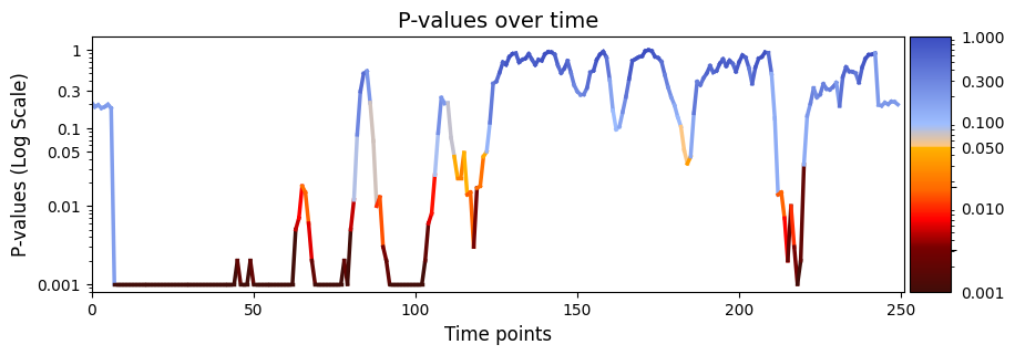
plot_heatmap from the graphics module.Note: Elements marked in red indicate a p-value below 0.05, signifying statistical significance.
[74]:
# The alpha score we set for the p-values
alpha = 0.05
# Plot p-values
graphics.plot_p_values_over_time(result_regression["pval"], title_text ="P-values over time",figsize=(10, 3), xlabel="Time points", alpha=alpha)
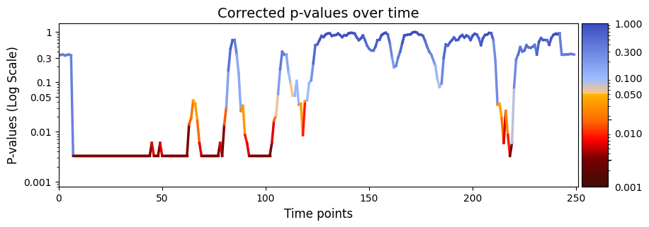
[75]:
pval_corrected, rejected_corrected =statistics.pval_correction(result_regression["pval"], method='fdr_bh')
# Plot p-values
graphics.plot_p_values_over_time(pval_corrected, title_text ="Corrected p-values over time",figsize=(10, 3), xlabel="Time points")
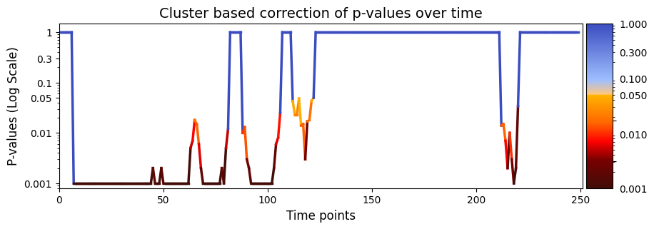
test_statistics_option=True while performing permutation testing, as it is an input to the function (pval_cluster_based_correction).[76]:
pval_cluster =statistics.pval_cluster_based_correction(result_regression["test_statistics"],result_regression["pval"])
# Plot p-values
graphics.plot_p_values_over_time(pval_cluster, title_text ="Cluster based correction of p-values over time",figsize=(10, 3), xlabel="Time points")
result_regression["pval"] correspond to the difference for each state over time for the two conditions. This will be done using the function plot_condition_difference.[77]:
# Detect the intervals of when there is a significant difference, will be highlighed
alpha = 0.05
intervals =statistics.detect_significant_intervals(pval_corrected, alpha)
# Plot the average probability for each state over time for two conditions and their difference.
graphics.plot_condition_difference(Gamma_reconstruct, R_trials, figsize=(12,3),vertical_lines=intervals , highlight_boxes=True, title="Average Probability and Differences (fdr_bh correction) ")

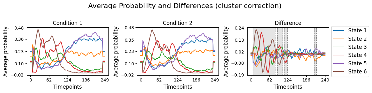
[78]:
# Detect the intervals of when there is a significant difference, will be highlighed
alpha = 0.05
intervals =statistics.detect_significant_intervals(pval_cluster, alpha)
# Plot the average probability for each state over time for two conditions and their difference.
graphics.plot_condition_difference(Gamma_reconstruct, R_trials, figsize=(12,3),vertical_lines=intervals , highlight_boxes=True, title="Average Probability and Differences (cluster correction) ")
Save the results
[79]:
io.save_statistics(result_regression, file_name="result_regression")
Statistics data saved to: c:\Users\au323479\Desktop\Permutation_test\GLHMM\Permutation_test_13-11_include_viterbi_path_permutation_matrix\result_regression.npy
Conclusion - Regression#
Our exampled involved presenting participants with two distinct stimuli across multiple trials spanning 10 different sessions. Permutation testing was performed across all trials within each session while while keeping the session order the same. The analysis generated the variable result_regression[“pval”], containing 250 p-values for each time point.
After correcting for multiple comparisons using Benjamini/Hochberg, significant differences were mainly in the early and mid segments of the signal (specifically, timepoints 7 to 83, 89 to 106 and 117 to 119) between state time courses (D) and stimuli (R).
The consistent occurrence of significant effects in the early segments of the recordings for every trial suggests a robust and reliable neural reaction at the onset of the stimuli. On the other hand, the decreasing significance towards the end of the signal may indicate a diminishing neural response to the presented stimuli over time. This temporal pattern in the results implies an initial heightened attention or processing of the stimuli, followed by a reduction in neural responsiveness as the trial progresses. The findings thus provide insights into the temporal dynamics of neural responses, indicating specific time windows of heightened sensitivity.
Across-trials within sessions testing - Correlation#
In correlation analysis, our goal is to find connections between predictor variables (D) and the response variable (R). Instead of explaining the variations in signal values over time, as in regression, our interest lies in figuring out the strength of the linear relationship between the state time courses (Gamma_reconstruct) and behavioral measurements, such as our stimuli. If the result is significant, it means that certain patterns in the state time courses (Gamma_reconstruct)
contribute to explaining the variability in behavioral measurements across trials. Now if the results is non-significant, it indicates that the observed relationship might just be a random chance. It means that our state time courses might not explain the variability in behavioral measurements.
across_trials_within_session function using correlation, input the variables Gamma_reconstruct (D) and R_session (R). Additionally, you can address potential confounding variables by incorporating permutation testing.method="correlation" to get the correlation coefficients and p-values.[80]:
# Set the parameters for between-subject testing
method = "univariate"
Nperm = 1000 # Number of permutations (default = 1000)
# Perform across-subject testing
result_univariate  =statistics.test_across_trials_within_session(Gamma_reconstruct, R_trials, idx_trials_session,method=method,Nperm=Nperm, test_statistics_option=True)
performing permutation testing per timepoint
100%|██████████| 250/250 [06:18<00:00, 1.51s/it]
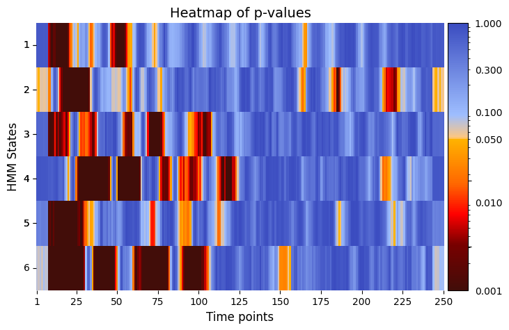
plot_heatmap from the graphics module.Note: Elements marked in red indicate a p-value below 0.05, signifying statistical significance.
[81]:
# Plot p-values
alpha = 0.05 # threshold for p-values
graphics.plot_p_value_matrix(result_univariate["pval"].T, title_text ="Heatmap of p-values",figsize=(8, 5), xlabel="Time points", ylabel="HMM States", annot=False, alpha=alpha)
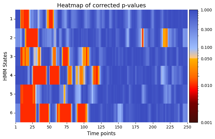
[82]:
alpha = 0.05 # threshold for p-values
pval_corrected, rejected_corrected =statistics.pval_correction(result_univariate["pval"], method='fdr_bh', alpha=0.5)
# Plot p-values
graphics.plot_p_value_matrix(pval_corrected.T, title_text ="Heatmap of corrected p-values",figsize=(8, 5), xlabel="Time points", ylabel="HMM States", annot=False, alpha = alpha)
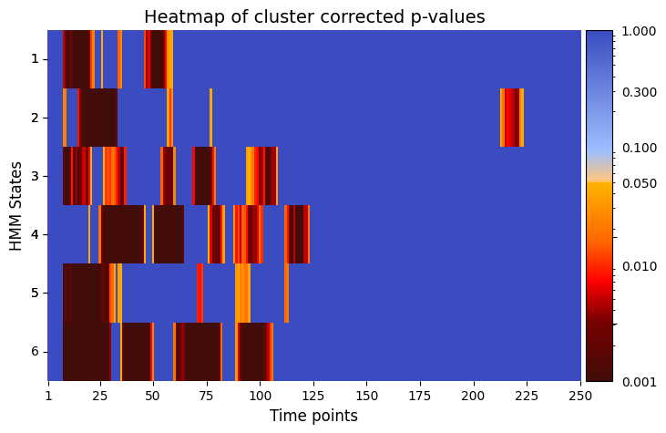
[83]:
pval_cluster =statistics.pval_cluster_based_correction(result_univariate["test_statistics"],result_univariate["pval"])
# Plot p-values
graphics.plot_p_value_matrix(pval_cluster.T, title_text ="Heatmap of cluster corrected p-values",figsize=(8, 5), xlabel="Time points", ylabel="HMM States", annot=False, alpha = alpha)
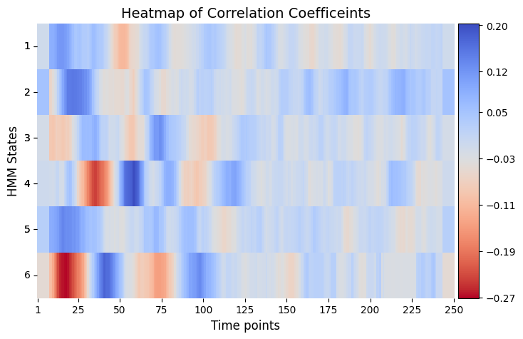
Plot Correlation Coefficients
[84]:
# Plot correlation coefficients
# Correlations between reation time and each state as function of time
graphics.plot_correlation_matrix(result_univariate["base_statistics"].T, result_univariate["performed_tests"], title_text ="Heatmap of Correlation Coefficeints",figsize=(8, 5), xlabel="Time points", ylabel="HMM States", annot=False)
Conclusion - Correlation#
In this example, the permutation testing analysis using correlation aims to study the relationship between state time courses and two different stimuli across multiple experimental trials. The resulting matrix, result_correlation["pval"], is structured as (time points x states), and it shows the trial-specific variations in the correlation between state time courses at every timepoint and the stimuli. Essentially, this matrix offers information about time-dependent and state-specific
correlation patterns.
When correcting the p-values using Benjamini/Hochberg or cluster based permutation testing, significant p-value for a specific HMM state and timepoint means that the correlation between state time courses at that timepoint and the stimuli significantly varies across experimental trials. This suggest that it is possible to pinpoint instances when changes in stimuli impact the state time courses, and thus highlight moments when stimuli induce observable effects on the state dynamics.
When looking at result_correlation["pval"], we observe time windows that shows a significant difference in the correlation between different HMM states and the stimuli. This can be interpreted as distinctive periods when specific neural states exhibit heightened responsiveness or susceptibility to the presented stimuli.