Across-Subject Testing with glhmm toolbox

This tutorial demonstrates how apply across-subject testing using the glhmm toolbox. We will use data sourced from the Human Connectome Project (HCP) S1200 Young Adult dataset (van Essen et al., 2013).

Make sure you have been granted permission to use the HCP data. If not, apply for such permission following the instructions in the HCP Data website. The HCP dataset provides an real-world context for this analysis and offers detailed information for each subject. Across-subject testing involves evaluating the connection between one or more HMM-related aggregated statistics and behavioral traits, such as sex and age or individual traits.

We’ll set up HMM-related aggregated statistics as the independent variable (D) and behavioral traits as the dependent variable (R). The objective is to assess the relationship between these variables.

Throughout the tutorial, we’ll guide you on applying the glhmm toolbox and drawing conclusions from the HCP dataset. While the setup of the glhmm toolbox may require some explanation, running the test itself is straightforward—simply input the variables D and R, and define the specific method you wish to apply. In this case, the methods include permutation using regression or permutation using correlation and is described in the paper Vidaurre et al. 2023.

Table of Contents

1. Load and prepare data

   • HMM-aggregated statistics

2. Across-Subjects testing

   • Family structure

   • Across subjects - Regression

   • Across subjects - Correlation

Install necessary packages

Let’s start by importing the required libraries and modules.

First, we will need to import the GLHMM-package as glhmm:

If you dont have the GLHMM-package installed, then run the following command in your terminal:

pip install --user git+https://github.com/vidaurre/glhmm

To use the function glhmm.statistics.py you also need to install the library’s:

pip install statsmodels

pip install tqdm

python -m pip install -U scikit-image

```

Import libraries

Let’s start by importing the required libraries and modules.

import os
import numpy as np
import pandas as pd
import glhmm.glhmm as glhmm
import glhmm.graphics as graphics
import glhmm.statistics as statistics

1. Load and prepare Data

For reproducibility and since the HCP dataset is very large, we provide the Gamma values (state probabilities at each timepoint) from a pre-trained HMM. If you don’t have these values, you can follow the instructions to train an HMM model in this tutorial from the glhmm toolbox.

Load Data Let’s start by loading the essential data for this tutorial: * Gamma: State probabilities at each timepoint exported from a fitted HMM model. The model is trained on HCP rest fMRI timeseries from 1001 subjects in the groupICA50 parcellation. * data_behavioral: Behavioral and demographic items from the same 1001 HCP subjects.

# Define the folder and file names
folder_name = "data"
data_behavioral_file = 'data_behavioral.npy'
data_gamma_file = 'gamma.npy'

# Load behavioral data
file_path = os.path.join(folder_name, data_behavioral_file)
data_behavioral = np.load(file_path)

# Load gamma data
file_path = os.path.join(folder_name, data_gamma_file)
data_gamma = np.load(file_path)

Explore data

Let’s take a closer look at the structure of the data.

print(f"Data dimension of data_behavioral: {data_behavioral.shape}")
print(f"Data dimension of data_gamma: {data_gamma.shape}")

Data dimension of data_behavioral: (1001, 2)
Data dimension of data_gamma: (1201200, 8)

The behavioral measurements, denoted as data_behavioral =[1001, 2], reveals that we have measurements for 1001 subjects. Each subject include information about their ‘sex’ and ‘age’.

Looking at data_gamma =[1201200, 8], we find that gamma measurements are concatenated for every timepoint across subjects (1201200 in total, corresponding to 1001 subjects by 1200 timestamps). The dataset comprises 8 columns, each representing the 8 different states at each timepoint per subject.

HMM-aggregated statistics

The purpose of the across_subject function is to conduct permutation tests between subjects. Like mentioned earlier, the data_gamma is a concatenated dataset across subjects and timepoints, totaling 1201200 data points (1001 subjects by 1200 time points) with 8 columns representing different states at each timepoint per subject.

To perform permutation testing using the across_subject function, we first need to compute HMM-related aggregated statistics. This involves deriving values that condense the states of the entire time series for each subject, resulting in a single set of values per subject (one row of data). Since we have gamma output from the HMM, we can calculate the Fractional Occupancy (FO). FO measures the duration spent in each state, providing the probability distribution for each state across the entire time series. As a result, each subject ends up with a single set of values that represents the states into a probability distribution that sums up to one for each subject.

Calculate indices

To calculate the FO from the gamma values, we must first specify the indices in the concatenated timeseries that correspond to the beginning and end of individual subjects or sessions. These indices should be organized in the shape of [n_subjects, 2] to precisely delineate subject boundaries within the concatenated timeseries.

To achieve this, we’ll use the function get_timestamp_indices. By providing the number of time points (1200) and the number of subjects (1001), the function outputs a variable in the shape of (n_subjects, 2). This variable contains the indices for the beginning and end of each subject’s scanning session.

# Prepare the number of time points and number of subjects
n_timepoints = 1200
n_subjects = 1001
idx_time = statistics.get_timestamp_indices(n_timepoints, n_subjects)

Let’s visualize the the first 5 time points

# Visualize the first 5 timepoints
idx_time[:5]

array([[   0, 1200],
       [1200, 2400],
       [2400, 3600],
       [3600, 4800],
       [4800, 6000]])

Calculate Fractional Occupancy (FO) Having obtained the necessary indices (idx_time), we can now proceed to calculate the FO using the glhmm toolbox.

# Calculate FO
FO = glhmm.utils.get_FO(data_gamma, idx_time)

Let’s take a closer look at the structure of FO and the behavioral data.

print(f"Data dimension of FO: {FO.shape}")
print(f"Data dimension of data_behavioral: {data_behavioral.shape}")

Data dimension of FO: (1001, 8)
Data dimension of data_behavioral: (1001, 2)

In this example, (FO) is a 1001x8 matrix and represent the distribution of the duration spent in different states across 1001 subjects. Each row of the matrix corresponds to a subject, and each column represents a specific state.

For example, if the FO matrix entry FO[i, j] is 0.2, it suggests that, on average, subject i spends 20% of the time in state j. These fractional occupancies provide insights into the temporal dynamics of the underlying states of the system across a population of subjects. It makes it possible to runderstand how subjects transition between different states and the overall patterns of behavior within each state.

Now, both FO and data_behavioral share the same number (N) of observations, aligning with the total number of subjects. As mentioned in the paper, the testing procedure involves a (N-by-p) design matrix, denoted as D, where p signifies the number of predictors. In our case, FO serves as the independent variable. Additionally, we have a matrix R with dimensions (N-by-q), representing dependent variables. In our context, data_behavioral fulfills the role of the dependent variable. Here, q signifies the number of outcomes to be tested.

Following this setup ensures a consistent and accurate testing process across our dataset.

2. Across-subjects testing

As we transition to the next phase of this tutorial, we will learn how to apply the across_subjects function to uncover relationships between the FO (D) and the corresponding behavioral variables (R) using permutation testing.

Permutation testing

Permutation testing is a non-parametric resampling technique that assesses statistical significance without assuming any data distribution. By randomly reshuffling measured data, it generates a null distribution, which can be used to test the null hypothesis—there is no difference or relationship between variables of interest to be tested. For the across_subject test it implies that each observation represents an individual subject, so we can shuffle or rearrange across subjects, as depicted in Figure 5A in the paper.

Figure 5A: A 9 x 4 matrix representing permutation testing across subjects. Each row corresponds to a subject, with one observation each. The first column: displays the original index of each subject (perm=0). Next columns: examples of permuted subject indices.

Family structure

By default, the across_subject function assumes exchangeability across all subjects, meaning any pair of subjects can be swapped. However, in reality, familial or meaningful connections between subjects may exist and can therefore violate the assumption that each subject are independent from each other.

To accommodate these connections, permutation tests with HCP data—or any dataset—involve creating the EB.csv file (Exchangeability Block). This file organizes data into blocks, each representing a family and makes it possibole to perform collective shuffling of entire families. For a more detailed explanation, refer to (Winkler et al, 2015). A tutorial on creating your EB.csv from the HCP dataset can be found in the glhmm toolbox here.

When using the across_subject function to consider family structure, you input a dictionary and we call it dict_fam. This dictionary specifies the directory to load the EB.csv file and includes optional parameters for running the permutation. In our example, we’ll use default options and solely define the file location of the family structure data (EB.csv).

dict_fam = {
    'file_location': 'EB.csv',  # Specify the file location of the family structure data
    # 'file_location': r'C:\Users\...\EB.csv'
}

Across subjects - Regression

In regression analysis, we are trying to explain the relationships between predictor variables (D_data) the response variable or signal (R_data).

Understanding Regression:

The objective is to uncover the factors influencing changes in our behavioral measurements. Specifically, we examine the amount of explained variance, it can be used to analyze whether the FO— representing the distribution of the duration spent in different states— significantly contributes to explaining the observed variability in behavioral measurements like ‘sex’ or ‘age.’ A significant result indicates that certain patterns in FO significantly contribute to explaining why the behavioral measurements varies. A non-significant result, on the other hand, suggests that the observed relationship can be attributed to random chance, implying that the FO may not play a significant role in accounting for the variability of the behavioral measurements (‘sex’, ‘age’).

Run the ``across_subjects`` function:

To run the across_subjects function requires providing inputs of FO (D) and data_behavioral (R). Sense we take family structure into account we will also include the variable dict_fam as an input. Additionally, you can account for potential confounding variables by regressing them out through permutation testing. To initiate regression-based permutation testing, set method="regression".

In this example, we will test how FO relate to variations in ‘sex’ and ‘age’.

# Set the parameters for between-subject testing
method = "regression"
Nperm = 1000 # Number of permutations (default = 0)
test_statistic_options = True
identify_categories = True
# Perform across-subject testing
result_regression  =statistics.test_across_subjects(FO, data_behavioral, method=method,Nperm=Nperm, dict_family=dict_fam, test_statistics_option=True)

C:\Users\au323479\AppData\Roaming\Python\Python39\site-packages\glhmm\palm_functions.py:1057: RuntimeWarning: overflow encountered in exp
  maxP = np.exp(lmaxP)

Number of possible permutations is exp(1586.6248450207656).
Generating 1000 shufflings (permutations only).

100%|██████████| 1000/1000 [00:00<00:00, 2826.30it/s]

We can now examine the local result_regression variable.

What we can see here is that result is a dictionary that contains the output of a statistical analysis applied using the specified method and test type.

Let us break it down: * pval: This array holds the p-values resulting from the permutation test. Each value corresponds to a behavioral variable and will have shape of 1 by q, see paper.

• corr_coef: Currently an empty list. It is intended to store correlation coefficients if correlation is involved in the analysis. In this case, the correlation coefficients are not calculated when we have set method="regression".

• test_statistic: Will by default always return a list of the base (unpermuted) statistics when test_statistic_option=False. This list can store the test statistics associated with the permutation test. It provides information about the permutation distribution that is used to calculate the p-values. The output will exported if we set test_statistic_option=True

• test_type: Indicates the type of permutation test performed. In this case, it is across_subjects.

• method: Specifies the method employed in the analysis. Here, it is 'regression', indicating that the analysis is conducted using regression-based permutation testing.

• Nperm: Is the number of permutations that has been performed.

Visualization of results

Now that we have performed our test, we can then visualize the p-value array.

We will import the function plot_heatmap from module helperfunctions.py

# Plot p-values
graphics.plot_p_values_bar(result_regression["pval"], title_text ="Barplot of p-values accounting for Famility structure",
                      figsize=(7, 3), ylabel="HMM states", alpha=0.05                      )

Conclusion - Regression

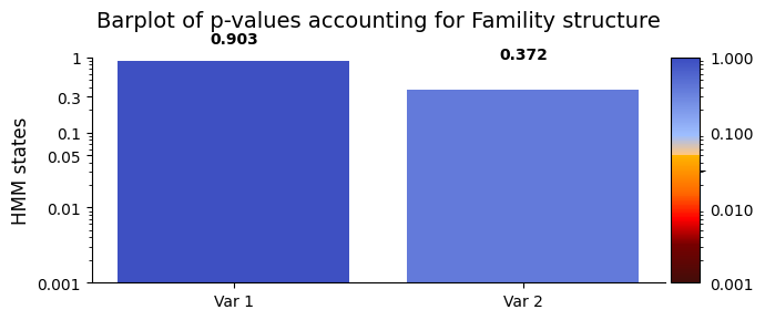
Each p-value corresponds to a specific test of the relationship between FO and the behavioral variables ‘sex’ and ‘age’. The permutation test for explained variance indicated that there is insufficient evidence to reject the null hypothesis for any of the HMM states. This suggests that, based on the statistical analysis, there is no statistically significant relationship among FO, ‘sex’and  'age' are not statistically significant for all states.

Across subjects - Correlation

In correlation analysis, our focus is on unraveling intricate relationships between variables. We can statistically assess the relationships between FO (R) and the behavioral measurements (D). A significant result suggests that specific probabilities of states in FO significantly contribute to the observed variations in ‘sex and ‘age. Conversely, a non-significant result indicates that the observed relationship might be attributed to random chance, and FO may not significantly influence the variability in ‘sex and ‘age.

Run the ``across_subjects`` function:

To run the across_subjects function we just need to provide inputs in the form of D-data (FO) and R-data (data_behavioral). Sense we take family structure into account we will also include the variable dict_fam as an input. To export the permutation distribution we set test_statistic_option=True. Additionally, we can account for potential confounding variables by regressing them out through permutation testing. To initiate correlation-based permutation testing, set method="correlation".

# Set the parameters for between-subject testing
method = "univariate"
Nperm = 10_000 # Number of permutations (default = 1000)
test_statistic_option=True
# Perform across-subject testing
result_univariate  =statistics.test_across_subjects(FO, data_behavioral, method=method,Nperm=Nperm,
                                                dict_family=dict_fam,
                                                test_statistics_option=test_statistic_option, identify_categories=True)

C:\Users\au323479\AppData\Roaming\Python\Python39\site-packages\glhmm\palm_functions.py:1057: RuntimeWarning: overflow encountered in exp
  maxP = np.exp(lmaxP)

Number of possible permutations is exp(1586.6248450207656).
Generating 10000 shufflings (permutations only).

100%|██████████| 10000/10000 [00:08<00:00, 1183.40it/s]

We can now examine the result_univariate variable.

result_univariate

{'pval': array([[0.469953  , 0.68543146],
        [0.20517948, 0.32336766],
        [0.18888111, 0.32986701],
        [0.51384862, 0.65423458],
        [0.30926907, 0.55234477],
        [0.26287371, 0.35136486],
        [0.2269773 , 0.94570543],
        [0.52084792, 0.21557844]]),
 'base_statistics': array([[-0.7529976 , -0.01307304],
        [ 1.28150949, -0.03635449],
        [-1.3511506 ,  0.03351405],
        [ 0.68191944, -0.01437657],
        [-1.07834326,  0.01901584],
        [-1.14513336,  0.03341424],
        [-1.18981512,  0.00236684],
        [ 0.6357729 ,  0.03923693]]),
 'test_statistics': array([[[7.52997603e-01, 1.30730431e-02],
         [1.28150949e+00, 3.63544906e-02],
         [1.35115060e+00, 3.35140475e-02],
         ...,
         [1.14513336e+00, 3.34142433e-02],
         [1.18981512e+00, 2.36683673e-03],
         [6.35772897e-01, 3.92369290e-02]],

        [[1.06668005e+00, 3.90441330e-03],
         [1.44240794e+00, 2.75625458e-03],
         [9.22922025e-01, 1.35853261e-02],
         ...,
         [1.06805531e+00, 2.82439016e-03],
         [2.20255705e+00, 8.37011017e-03],
         [4.37315726e-01, 1.86695328e-03]],

        [[6.61097808e-01, 2.72188732e-02],
         [7.74908794e-01, 3.15968328e-02],
         [1.22213771e+00, 6.60544623e-02],
         ...,
         [5.22669805e-01, 1.02306052e-02],
         [1.33125487e+00, 2.65548421e-02],
         [7.64713715e-01, 3.66078678e-02]],

        ...,

        [[1.28931272e+00, 4.26791749e-02],
         [9.73283022e-01, 3.41931274e-02],
         [1.10301327e+00, 1.94661123e-02],
         ...,
         [3.54691932e-01, 2.80091297e-03],
         [1.39112699e+00, 2.57275584e-02],
         [2.58279078e-01, 2.32332320e-02]],

        [[2.18538920e+00, 6.73309864e-02],
         [1.28690386e+00, 3.47850438e-02],
         [2.98976074e-01, 2.83774959e-02],
         ...,
         [3.07891753e-02, 3.29632644e-02],
         [1.27231115e+00, 5.75689338e-02],
         [4.02767339e-01, 2.86424215e-02]],

        [[6.83460832e-01, 1.96811509e-02],
         [1.22536278e+00, 5.50794400e-02],
         [9.98663010e-01, 3.89226042e-02],
         ...,
         [7.86289071e-01, 7.59862335e-02],
         [5.98438676e-01, 5.97783842e-02],
         [2.99530189e-01, 1.18797389e-04]]]),
 'test_type': 'test_across_subjects',
 'method': 'univariate',
 'test_combination': False,
 'max_correction': False,
 'performed_tests': {'t_test_cols': [0], 'f_test_cols': []},
 'Nperm': 10000}

Visualization of results

Now that we have performed our test, we can then visualize the p-value and correlation matrix.

We will import the function plot_heatmap from module helperfunctions.py

# Plot p-values
alpha=0.05 # p-value threshold
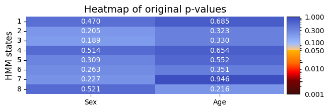
graphics.plot_p_value_matrix(result_univariate["pval"], title_text ="Heatmap of original p-values",
                      figsize=(7, 2), ylabel="HMM states", alpha=alpha,
                      xticklabels=["Sex", "Age"],normalize_vals=True)

Plot permutation distribution

Presented here are the significant test statistics of our permutation distributionfor the different states. The red line shows the observed statistic, while the datapoints of the histogram represent the permutation distribution

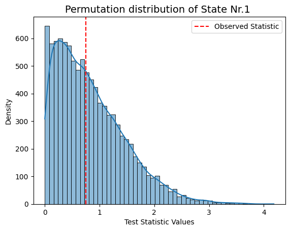
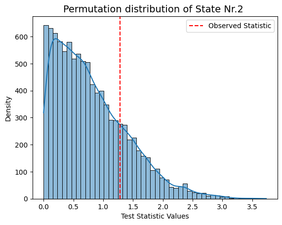
# As we didn't find any significant values we can print out the permutation distribution
# Visualizing the permutation distribution for sex, which got index=0
for i in range(result_univariate["test_statistics"].shape[1]):
    graphics.plot_permutation_distribution(result_univariate["test_statistics"][:,i,0],title_text=f"Permutation distribution of State Nr.{i+1} ")

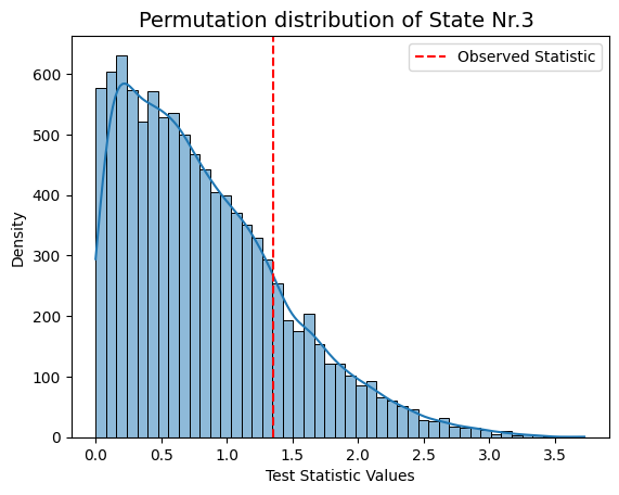
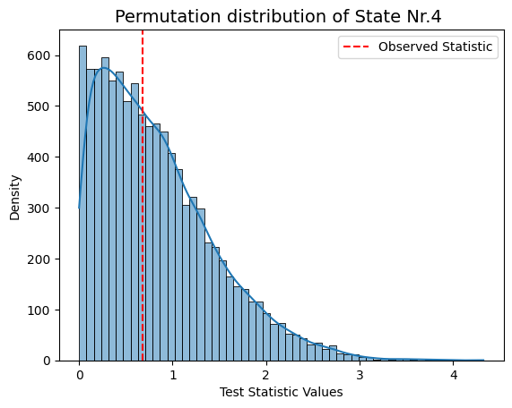
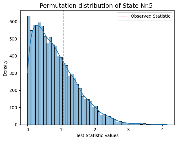
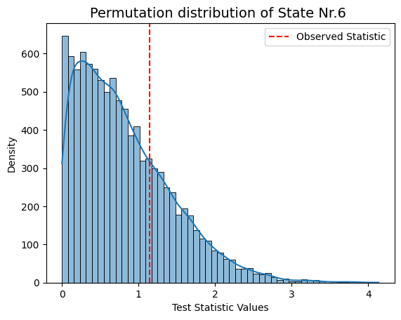
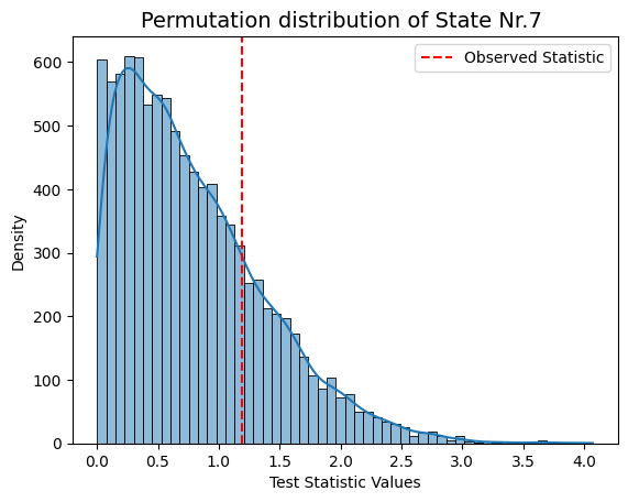
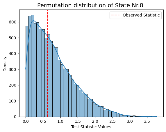
Conclusion - Correlation

Following permutation testing on correlation across different HMM states derived from FO, the results indicate no statistically significant correlation with the behavioral measurements for 'sex' and 'age'. With a predetermined alpha value of 0.05, none of the p-values in the matrix fall below this threshold. This suggests that, within the permutation testing framework, there is no evidence to reject the null hypothesis for any specific HMM state.

What is interesting is that the findings align with the null relationship observed through an alternative prediction approach, which is also part of the GLHMM toolbox. This approach involves predicting age and classifying sex based on all states’ FO, switching rates, and lifetimes (link).

Notably, the correlation between model-predicted and true age values is below 0.1, and the accuracy for predicting sex is approximately 60%, just above chance. This implies that if we can’t predict age or sex from the comprehensive summary statistics of all states, including FO, switching rates, and lifetimes, we wouldn’t expect individual states’ FO to exhibit significant correlations with age and sex.

Essentially, despite employing different methodologies, both permutation testing on correlation and the prediction approach concur—there is no strong relationship between HMM summary statistics and age/sex. This consistency is encouraging as it suggests that the permutation test effectively captures the absence of significant correlations in the Human Connectome Project (HCP) dataset.